Day 46

Scrutinizing yesterday’s approach

The method yesterday took a quantile approach at creating a prediction interval. I read the blogger’s explanation a bit further and I finally have some trust in his approach.

This statement still bothers me though:

A prediction interval is an estimate of an interval into which the future observations will fall with a given probability. In other words, it can quantify our confidence or certainty in the prediction

I have my doubts about how well that concept is represented by the method they propose. future outcomes, however I don’t know that this is the case. I would imagine that each tree is more or less following a similar path and is not capable of predicting the full range of possible response values. What if none of the trees are able to predict a certain response value?

Also you can only be 100% confident in an interval that spans the entire y-axis, while this method will give you a much narrower region that only spans the range of values predicted across all the trees.

I just found this from the community scikit-learn docs that claims to add confidence interval calculations to scikit-learn RF through a module called randomforestci.

The official PyPi release of randomforestci gave me an error when I tried running fci.random_forest_error() because the documentation online is for the development version (v. 0.2), different from the official release (v. 0.1). The order of the arguments was different, so I instead installed the development version.

However I was still getting errors, this time from NumPy function calls. The problem seemed to stem from the fact that I have multi-dimensional output.

To the source code

I looked through the source code and found the area that was throwing the error. By manually running bits of the function line by line I was able to narrow down the root of the issue.

I modified this section:

pred = np.array([t.predict(X_test) for t in forest])
pred = pred.reshape(pred.shape[0],-1).T

Previously it was creating a 3D matrix (retaining the daily seperations) but I removed the seperations and just created a stream of power values (kind of like how I ravel() the predicted values before I plot them).

To do this I copied the random_forest_error() function from the source code, prepended fci. to its internal function calls and edited the region I showed above.

Now the code will run properly, but I think something is still wrong. At some points the variance it reports is negative which is illogical. While reshaping the array might have stopped the computational error, I probably caused some of the calculations to become invalid. I don’t know enough about their calculation technique to tell for sure what part is invalid. It’s probably not worth trying to fix their implementation. In the meantime I opened an issue for it on the GitHub source.

Confidence intervals vs Prediction intervals

It’s important to differentiate between the two. This page does so in an understandable way. Prediction intervals are broader in that they account for both variance in the sample and variance in the predictions (as the page states, prediction intervals are larger than confidence intervals). I think for my purpose, prediction intervals would be more appropriate.

Tweaking the old method

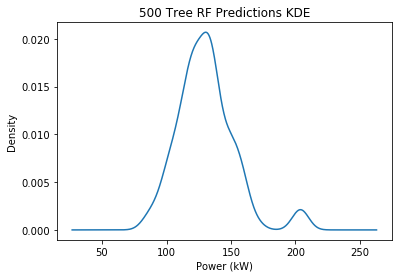
One thing I wanted to quickly verify was how representative the trees were of all possible predictions. I increased my forest size to 500 and plotted the distribution of predictions for a single output value (first element of the first output):

By no means a perfect normal distribution, but it looks better than the sparse distribution of my smaller 50 tree forest. I know that the parent RF estimator returns the mean of these values, so I could take their standard deviation as a way to estimate the population variance and assume normal distribution. Or could I continue with the percentile-based approach. The benefit of the newer method is that it has no size limit so it’s fairer at large prediction intervals (i.e. 100% prediction interval is infinite)

Here’s the full threshold calculation:

pred = np.array([t.predict(X_test) for t in est])
sd = np.std(pred,0).ravel()
quantile = 0.95
z_max = norm.ppf((quantile+1)/2)
y_thresh = y_pred + z_max*sd

And here’s a resulting plot with 100 trees:

It’s a bit different from the plot I had yesterday (the threshold has moved up in some areas). I’m satisfied with it for now.

In the future I may want to consider standardizing the residuals so that when I report the potential energy savings it’s not overinflated in areas of high variance.

Starting the abstraction

My scripts have all been very specific but I want to start generalizing the functions.

I spent the rest of today laying some groundwork for a function to create the RF model:

def make_model(target_vals,target_features,input_size,gap_size,output_size):   
    n = len(target_vals)
    ixs = np.array(range(n))
    ix_windows = egz.rolling_window(ixs,
                                input_size
                                + gap_size
                                + output_size,
                                output_size)
    X_ixs,_,y_ixs = np.split(ix_windows,[input_size,input_size+gap_size],1)
    X = np.concatenate((np.array([target_vals[ixs] for ixs in X_ixs])[:,::int(egz.pp_day/24)],
                    np.array([target_features[ix] for ix in y_ixs[:,0]]),
                    ),1)
    y = [target_vals[ixs] for ixs in y_ixs]
    est = RandomForestRegressor(n_estimators = 50)
    est.fit(X,y)
    return est

I was trying to figure out how to simplify the creation of the feature matrix. Since there’s two main sections (part based on previous results and part based on properties of the target day) I split up the parameters, one for the historical/output data (target_vals) and one for extra feature properties (target_features). I would just call them vals and features but the values have a dual usage, partly as features and partly as training targets.

The setup could be used alongside a dataframe containing properties about each power entry (e.g. occupancy, time of day, month, etc.) although most of those properties could be calculated at runtime rather than storing them in advance.