Day 43
Aug 4, 2017 · 890 words
Setting up the input/output
Cluttered approach
First I split the data up into hourly chunks with the rolling_window method. Then I run a 2D rolling window to pull enough hours to include both my predictor value and response values. Note that there’s extra data in the middle. I drop this middle section and assign the X and y arrays via np.split(). Then I reshape the arrays so that the hours are no longer divided. I’m using the rolling_window method that I mentioned yesterday (using strides) and a 2D version that doesn’t use strides as defined here.
data = egz.df_energy['Main (kW)']
bins = egz.rolling_window(data,4,4)
windows = egz.rolling_window2D(bins,24*7*5+1)

X,_,y = np.split(windows,[24*7*4,24*7*5],1)

X = X.reshape(X.shape[0],-1)
y = y.reshape(y.shape[0],-1)
Streamlining it
I can declutter this process by getting rid of the step where I break into hour-long bins (although that section did make it a bit easier to follow):
windows = egz.rolling_window(data,4*(24*7*5+1),4)
X,_,y = np.split(windows,[4*24*7*4,4*24*7*5],1)
See below for a more readable edit
The result
Now my X array of 4-week predictor values starts at 00:00:00 on 8/5/15 and my y array holds the hour-long predictions 5 weeks from then starting on 9/9/15 at 00:00:00.
4 weeks of prediction data, 1 week gap, 1 hour of target data.
Null values
Apparently sklearn doesn’t like when you give it null values. For now I’ll just fillna(0) although this may impact the accuracy of the model. I’d be better off filling in values from the week before to give a better estimate of the actual usage that occured then (or average the value the week before with the interpolated values to also reflect that day’s context).
Making predictions
Here’s a really big plot of all the test samples compared to their target values. Since the predictions are each hour-long bins of data, I plotted them by raveling the predicted array.
Click the image to expand it to full size:
Measuring the fit
I tried measuring the Mean Absolute Percent Error to measure the fit, however the outlier days when the model didn’t know that there was no school threw this measure off entirely (it was over 4 billion percent).
To reduce the impact of these outlier days I instead measured the Median Absolute Percent Error which gave a much more reasonable value. Note the addition of a 1e-9 term so that the system doesn’t try to divide by zero.
np.median((np.abs(((y_test+1e-9) - (pipe.predict(X_test)+1e-9))) / (y_test+1e-9)))
>>> 0.16049520499889364
To put this in comparison, the MIT report from yesterday measured a MAPE of about 0.12 for RF and 0.14 for ANN, so we’re not far off. And this is only trained on data about previous consumption, so it doesn’t have information about holidays yet.
Changing variables
I tweaked the ranges of some of the window variables to see how it affected the predictions. To do so I added some more variables which also makes the assignment more readable:
input_size   = 4*24*7*4
gap_size     = 4*24*7
output_size  = 4

windows = egz.rolling_window(data,input_size+gap_size+output_size,output_size)
X,_,y = np.split(windows,[input_size,input_size+gap_size],1)
| Input | Gap | Output | Median APE |
|---|---|---|---|
| 4 weeks | 1 week | 1 hour | 0.1605 |
| 1 weeks | 1 week | 1 hour | 0.1718 |
| 4 weeks | 1 week | 1 day | 0.1597 |
| 8 weeks | 1 week | 1 day | 0.1717 |
| 8 weeks | 1 day | 1 hour | 0.1439 |
| 8 weeks | 1 day | 1 day | 0.1569 |
| 4 weeks | 1 day | 1 day | 0.1593 |
| 4 weeks | 1 day | 1 hour | 0.1325 |
| 1 weeks | 1 day | 1 hour | 0.1526 |
| 1 day | 1 hour | 1 hour | 0.0794 |
Note that due to the random nature of the model, the accuracy is subject to change across trials (but as an ensemble method it should be somewhat consistent).
As expected, the model with the smallest gap (1 hour) had the best accuracy but at that small of a gap the forecast is no longer very useful. From what I can tell, the winner is 4 weeks of input, 1 day gap, 1 hour predicted. That way the forecast will be available a day beforehand. We could also present the user with an option to run a forecast of their desired length, although they would have to wait for the server to process their request.
Better handling of null values
Instead of replacing the nulls with 0 kW, I can replace them with last week’s value with
data.fillna(data.shift(-4*24*7))
I actually tried using the 'W' offset alias instead of calculating the week index interval but it wasn’t behaving as I expected.
Slow training
The training process is rather slow, even if I drastically reduce the number of samples. It appears the biggest time-suck is the large number of features that need to be tracked.
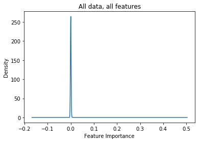
The feature_importances_ property of a trained RF estimator shows the relative importance of your features. Here’s what the distribution looks like:
As you can see, almost all the features have close to zero importance. Here’s the top 10 values of the sorted list:
| Index | Importance |
|---|---|
| 2114 | 0.335970 |
| 2687 | 0.107384 |
| 2115 | 0.096686 |
| 2113 | 0.050099 |
| 97 | 0.043213 |
| 96 | 0.031255 |
| 98 | 0.024074 |
| 2116 | 0.014845 |
| 99 | 0.011222 |
| 2208 | 0.006476 |
The importance drops off very quickly. Only a couple of sparse values are significant predictors (the top contenders appear to be from a few weeks in the past).
By changing the max_features argument to something like 'sqrt' or 'log2' I was able to increase the training speed at the expense of the median APE (0.13 vs 0.15).
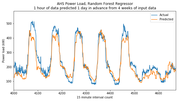
Here’s an example output using 'sqrt' max features:


