Day 41

Multi-step forecasting

I quickly corrected it after posting, but I mistakenly thought I had struck gold last time when working with lagged features. In reality, I was violating the rules of predictions by including data about the future in my testing inputs (I was performing a bunch of one-step-ahead forecasts which made it look like my overally forecast was really strong).

When I tried recursively generating lagged predictions for my inputs, I got a much weaker model. In fact, I found that the lag features only hurt my overall model compared to solely accounting for current conditions. At the moment I don’t have a whole lot of hope left for the multiple regression approach, but the problem may lie in my naive attempt at multi-step forecasting. This page explains a few different techniques (I was using the recursive one).

I’m particularly interested in the final method (multiple output approach) which uses a model which predicts an entire span of time rather than a single prediction value. It does so by training the model on multi-dimensional outputs, something I’ve not yet tried. For instance, I could train a model to predict the entire next day’s power usage based on the past week.

In order to do this I’ll want an array of rolling window measurements. Unfortunately the Pandas rolling objects don’t appear to have a handy way to return their underlying array structures.

Data involved

For now I’ll only consider lag data, not features about current time. To see how far I can push it, I’ll have my input be an array of all of the data for the past 4 weeks, and my output be an array out the data for the next week. To generate this from my regular time series I made a helper function:

def train_target_windows(arr, windows, step=1):
    trains = []
    targets = []
    for i in range (len(arr) - windows[0] - windows[1] + 1):
        trains.append(arr[i:i+windows[0]:step])
        targets.append(arr[i+windows[0]:i+windows[0]+windows[1]])
    return (np.array(trains),np.array(targets))

Here you pass in your starting array arr and a tuple of desired window sizes for your input/output sets. For me this was (4*24*7*4, 4*24*7) (i.e. 4 weeks, 1 week). The step parameter lets you take larger steps between values on the input matrix to reduce the number of features that need to be regressed.

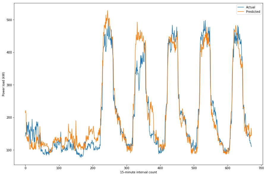
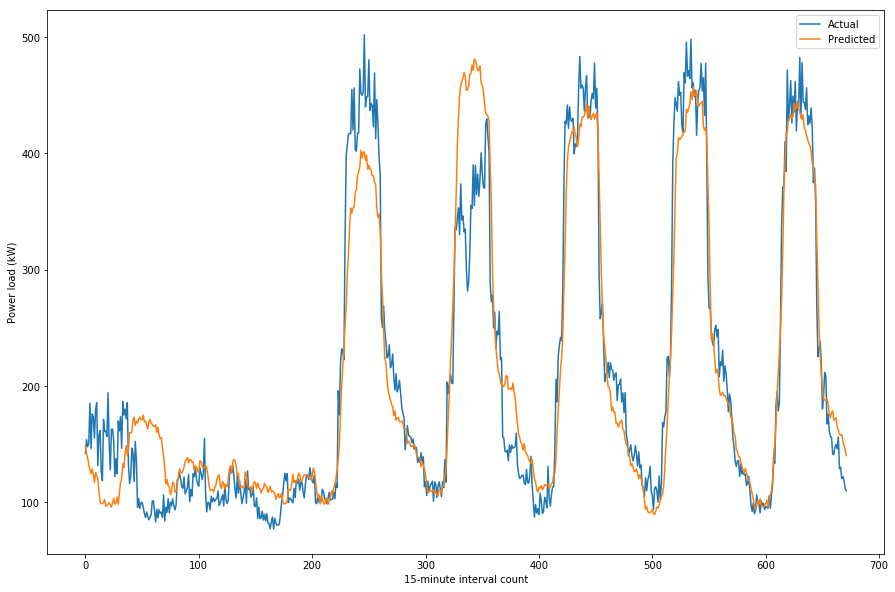
Here’s what I got when training a DecisionTreeRegressor model on windows extracted from 10,000 of the data points:

>>> est.score(X_test,y_test)
0.59252701026688193

And here’s the same calculation with a RandomForestRegressor:

>>> est.score(X_test,y_test)
0.80756960256071542

Not bad. I’m just using the parameter defaults here since I don’t know enought about these predictors to know what parameters to change. And this time I’m not cheating when I make this prediction. That entire week of data is predicted from the previous 4 weeks in 1 calculation, so there’s no funny business where I’m using future values within the prediction input.

Right now the code is pretty slow (takes a minute or so to run), mostly due to the slow window generation step. Currently I’m making a lot of windows with a lot of unecessary overlap so that’s one area I know for sure I could improve.

Realtime anomaly detection

Remarks on the studies

I’m impressed by the results of Chou & Telaga in their study on realtime anomaly detection. They tested 2 methods, ARIMA and NNAR on two sizes of sliding windows. Overall, the best predictor was NNAR on a 4-week window of training data. Both NNAR tests performed better than the ARIMA tests.

I was under the impression that we would need a large span of data in order to make an accurate model so it’s a nice surprise that only 1 month of prior data may be necessary for training. That also means calculations can run much more quickly.

One thing to note is that for their study they had a data stream at 1-minute intervals, while the data I have for testing is at 15-minute intervals. I’m not sure how significantly this will affect my results.

Lastly, they used the R language in their study. It may be worthwhile to try this if there are no equivalent functions for the methods they used in Python. The methodology report was most recently revised in January 2014, and the subsequent report using it for an early warning application was revised in January 2017. So the technique had been implemented fairly recently and has stood the test of time.