Day 4

I did some searching about median absolute deviation in pandas and found this post. The devoper mentioned that they were considering adding a center parameter to the built in Pandas.Series.mad() function, but advocates against using the function altogether and instead just implementing median absolute deviation manually like this:

abs(x - x.median()).median()

In my case, I’ll be using x_right - x.median() since I’m only looking at the upper values.

In the context of my own code:

night_mad = abs(s_night_right - night_med).median()

Which comes out as:

In [1]: night_mad
Out[1]: 20.2772

Side note, when calculating the MAD with all the data instead of just the right side, I got 18.7547 which is just a bit smaller.

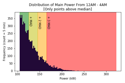
After some time reading the matplotlib documentation, I was able to generate the following chart:

I added shaded regions to highlight the areas formed by various multiples of the MAD. When working with a normal distribution, you would consider points that are more than 2 standard deviations (SDs) away from the mean to be unusual and those more than 3 SDs to be very unusual, since less than 1% of points should occupy that area. The MAD is not a direct equivalent to the standard deviation, so we can’t just use the same indicators for it. Yesterday I mentioned a constant factor of 1.4826 that can be used to approximate the standard deviation of a normal distribution. I can’t be sure exactly what kind of distribution to expect here, but for now I will just pretend that we should expect a normal distribution, at least for the right side of the data. And if we assume that, we can also assume that the mean is the same as the median.

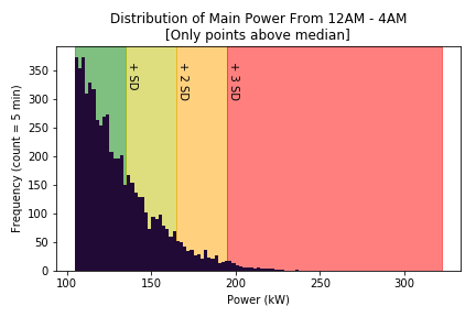
Here’s the same plot but with the estimated standard deviations as region bounds instead of plain MADs. The value of $\hat{\sigma}$ came out to 30.063.

Visually, it looks like a pretty good way to see which regions contain values that are too large. But statistically, I’m not too sure of its validity. It’s really a judgement call of whether the population is supposed to be normal or not. I’ll have to test it out on other samples to see if it still holds up.

Gaps in the data

It recently came to my attention that the parsed data is not a perfectly continuous stream. It starts off fine, but as the data goes on there are some missing points. Eventually it becomes half as dense as it started out, with measurements for only every other timestamp. I need to keep that in mind when performing these calculations. I think that this is not going to be an issue for the time being, because even though parts of the data are less populated they still should show a similar distribution.

Pandas has a guide for how to work with missing data points in your code. Going forward, I can use notnull() and isnull() to filter such points out of my dataframe/series. For example, the basic line plot goes blank when trying to plot between empty values.

Status Update

At this point given a CSV input file I can select a column and create a series of the entries that are more than 3 estimated population standard deviations away from the estimated population mean. The validity and usefulness of this measure is still yet to be tested. It’s a good start though. In the future, I hope to refine my understanding of the expected model for the population. At this point I’m trying to mold the right side of the sample into a normal curve and comparing against that. But perhaps it would be better to use the left side as a model and mirror it over to the right side. Or maybe I should be taking the MAD of the entire sample instead of just the right side. These are things I will have to keep in the back of my mind.

Outliers are just one piece of the puzzle though. We’re not just looking for single days where there was an overuse of power, we’re looking at overall ways to reduce power. Perhaps the data is not centered where it should be. It is challenging to determine where the center of a sample should be. We want the analysis to be able to handle many different types of buildings. Some might actually require much power. That is, given two samples with similar centers, we should be able to detect which one is normal and which one is not. I think to do so, I’ll want to somehow use the lower end of the sample as a reference point.