Day 38

Today is a shorter post as I have to leave this afternoon.

Testing the cross validated results

Last time I noted that the initial scores I was seeing didn’t appear high. Today I’m going to look deeper into how to interpret the results. I think last time I was just looking at night data but today I’m going to use the school data (which gets an even lower score on the testing set, below 30%)

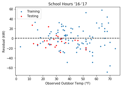
Plotting the residuals

The first area I should look is the residual plot to see if there are any unwanted trends

I see a couple of things here:

• There’s more variance for the higher temperature values
• The testing residuals are mostly negative

The latter issue could just be poor luck (more data would help create a stronger prediction on future test points). The former could be a real problem.

Nonconstant variance

My analysis of the residual distribution (i.e. how I’m going to tell which points are too far from the trend) relies on the assumption that the variance is independent of the explanatory variable. I wouldn’t want to end up solely flagging summer data points as abnormal just because there is more variance on hotter days.

This presentation looks at the effects of nonconstant variance, also called heteroscedasticity. Heteroscedasticity violates the assumptions of OLS, but the presentation notes that using a more robust estimator such as Huber regression makes this less of an issue.

Since my residuals “fan out” in a predictable fashion I could apply a transformation to the response variable to make the variance more constant. My concern is, what if the heteroscedasticity is not so predictable (e.g. what if it oscillates between low and high variance rather than a constant increase)?

I have to cut this post short as I’m leaving for a weekend trip. Next week I’ll be back to continue where I left off.