Day 35

EDIT: as a disclaimer, this post’s use of normalization is flawed. The subsequent post revises this error.

How much error is acceptable?

Before I get much further refining the regression technique, it’d be good idea to spend some time figuring out how I’m going to end up using it. The obvious use of regressions is to allow me to find an expected value given certain arguments, but I’m not expecting the sample to fit these predictions exactly. Considering the small random variance in power usage under a given set of parameters, you can assume the residuals should follow a consistent distribution.

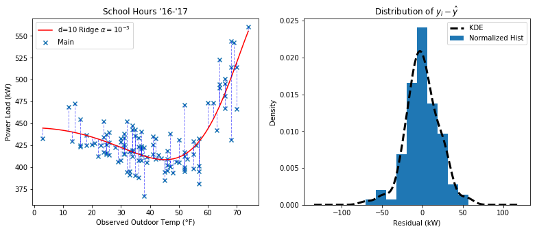
Here’s a look at the distribution of residuals in a Ridge regression of the power versus temperature data during school hours

Distributions to Consider

The usual assumption is that the errors (and residuals) should follow a normal distribution.

Previously, I went with the assumption that our response variable follows a lognormal distribution due to the lower bound of power usage. If I continued that assumption, then I think I would have to log-transform all the data before the whole fitting / residual calculation process, and from then on I could treat it as normal.

I also might want to consider a Student’s t-distribution in stratifications of the data where there are less than 30 data points. Here I have 114 so it is probably not necessary.

I think for now I’ll stick with assuming normality since it’s the most straightforward. There may be negative implications of log-transforming the regressors that I haven’t considered.

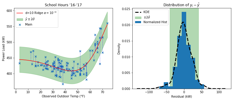
Here I added shaded regions to highlight the area that is predicted to enclose 95% of the data assuming normality.

Note that $\hat{\sigma} = \sqrt{ \frac{1}{m} \sum_{i=1}^{m} (y_i - \hat{y})^2 }$, or in other words the variance equals the mean sum of square errors of the residuals. $\hat{\mu}=0$ since in an ideal normal distribution the positive and negative residuals would all cancel out.

At first glance it appears that the acceptable region gets narrower on the right, but this is just a visual side effect of the steep slope of that area (like a caligraphy pen). The height of the shaded region is constant all the way through.

Note for the future: It might be better to use a more robust stastic like a scaled MAD for estimating the underlying standard deviation of the residuals

Difficulty implementing robust estimators

Right now the model gets completely thrown off in the face of large outliers. We don’t have huge outliers but if our sample has any abnormal power usage, the model is being impacted by it, making it harder to detect abnormalities. To reduce this effect I looked into this resource on robust linear estimators.

I tried all the estimators they describe (RANSAC, TheilSen, and Huber), and each one had a poor fit on the data (even at lower polynomial degrees). At higher degrees they weren’t even close. Part of the issue is that as far as I can tell, Huber regression is the only one that incorporates regularization (it’s related to Ridge regression).

Aside from that, I wonder if normalization has something to do with it? Yesterday I noticed that I had to set normalize=True to get the basic regularized estimators to fit properly. There is no such parameter for the robust estimators, but there is a preprocessing Normalizer(). I thought I could just toss it into the pipeline to replicate the behavior of the normalize parameter, but on trying this with the Ridge regressor I got very different results (I also tried both norm arguments).

What exactly is normalization?

Generally, normalization scales a set of values so they all lie between 0 and 1. Using l2-norms, this would scale a vector to be of unit length. In my Calc 3 course we used this method to find unit vectors, though we never actually called it normalization. If using the l1-norm, I believe it scales the vector so that its values sum to 1 (i.e. its l1-norm = 1). The default method of the Normalizer() prepocessor is to use the l2 norm.

One odd thing I noticed is the Normalizer tranformation object introduces more calculation error than the non-class-based preprocessing.normalize() method (assuming the numpy.linalg.norm() method is accurate). The former consistently scales the input vectors at least $10^{-4}$ units too high (e.g. 1.000159…), while the latter isn’t more than $10^{-15}$ units lower than it should be (e.g 0.99999999…). Still, I don’t know if that’s enough to be causing my troubles. I tried manually using the normalize() method rather than putting the Normalizer() in my pipeline and I didn’t see any noticable change in the output plot.

The solution

The moment of truth… did this actually help fix the bad plots from the robust estimators? Yes and no. RANSAC and TheilSen still completely break at high order polynomials since they don’t have regularization. Huber regression is performing wonderfully though. I tested it out by tossing in a ridiculously high outlier at 10,000 kW and Huber didn’t even flinch. It’s not worth trying the debug the other two estimators when Huber does the job just fine. I’m happy with it, as judging by its description it’s a relatively noninstrusive method that softly aids in reducing the impact of outliers.

Putting it in the pipeline

Sklearn lets you make custom transformer functions using preprocessing.FunctionTransformer. For my function I used preprocessing.normalize, and I passed the keyword argument to set axis=0:

myNormalizer = FunctionTransformer(normalize,kw_args={'axis':0})

Then I can just put myNormalizer in the pipeline after my PolynomialFeatures transformer and it will properly normalize my features for estimators that don’t support the normalize parameter.