Quick Disclaimer on Validation

For now I’m testing models using all the data available. Later on I will worry about proper validation / cross-validation procedures.

Power vs. Time of Day

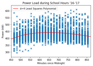
I have already looked at the load profile of the school throughout the day (see Day 17), but that was using a fairly simple method that relied on the fact that the data is being sampled at the same 15-minute intervals every day. It only considered the midpoint of the data at each 15-minute timestamp, so the trend line had total freedom to jump around as much as it pleased. It would be more useful to fit a regression to the load profile to capture a smoother, more generalized model.

Since they’ll be used in the regression calculations, I’ll need to convert the timestamp objects to quantitative values. I’ll measure the number of minutes since midnight. An easy way to get this is:

data.index.minute + data.index.hour*60

Using the same polynomial fitting method from yesterday:

Robustness of the Regression

I often bring up the fact that we’re assuming flaws and outliers in our sample, which is why I have leaned towards measures like the median and MAD over mean and standard devaiation. The least squares regression technique tries to minimize the overall cost function, but that means it isn’t resistent to outliers in the data. It just wants to “please” all the points equally by picking a middle ground of “maximum likelihood”.

Wikipedia has an article on alternative robust techniques. The overall best compromise of effectiveness and efficiency seems to be the MM-estimation.

The SciPy documentation also has a post that overviews how you can go about robust nonlinear regression. It notes that the absolute loss (AKA Least Absolute Deviations or LAD) is a robust loss function, but it is more complex to optimize than least squares (since it is non-differentiable). Instead it describes applying a sublinear function (which grows slower than a linear function) on the cost function

Note: I’ve found many scipy.optimize functions that seem to accomplish the same task (leastsq,curve_fit, and least_squares) but from what I’ve read the most recent and direct version is least_squares, which is what is used in the post I linked above

Kernels?

I haven’t found a clear offering in the “Big 3” libraries I’ve used (Pandas, NumPy, SciPy) for kernel smoothing. It’s appealing that kernels let you use complex features without explicitly defining them, but so far our data has’t appeared to follow too crazy of a model anyway. The most complex model I can imagine us using would be something that models the entire lifespan of the time series power data, but we might be able to simply fit that using sinusoidal features (to account for the daily and annual cycles).

Realistically, we won’t even need to make that kind of complex model because we could just perform seperate regressions on subsets of the data filterd by factors such as day of the week, week of the year, temperature, etc. which would be causing those hourly or seasonal shifts. We could allow the user to check off boxes for which factors they want to stratify the regressions by. Each stratified regression could most likely be fitted by a low degree polynomial.

scikit-learn

I’ve been seeing the name scikit-learn pop up a lot in my research lately (such as in my search for kernel smoothing), so I finally checked it out. It’s a library built on Numpy, SciPy and Matplotlib designed for machine learning. It can do classification, regression, validation, and tons more. Plus it’s supported by Anaconda. I’m definitely going to poke around the documentation and see what it can do for us. This resource provides tutorials that go over the key points. I’ll just make some notes of anything interesting I see along the way.

Unsupervised learning & Clustering

So far I’ve just been looking at supervised learning which looks for patterns according to a provided set of inputs and outputs. Unsupervised learning on the other hand finds patterns based solely on input vectors. This goes way back to when I mentioned that it would be nice to be able to automatically classify different power usage profiles (e.g. night, weekend, school day, special event) rather than having the user manually specify them. Unsupervised learning is the general topic, clustering is a more specific category that applies to what I’m talking about here.

Using estimator objects

Using models in scikit-learn is amazingly straightforward. There are various estimator object types (e.g. for linear, polynomial, kernel, and many more) which have a simple fit() method that takes in the input and response values, and a predict() method that takes in a new value and predicts the response based on the model. Machine learning is a really complicated subject but this library practically spoonfeeds it to you; it’s fantastic.

Picking estimators

You can use folding methods such as k-folding to perform cross-validation on your “learning” data set to narrow down the best parameters for your estimator. (Estimators actually have a score method that indicates how well they fit the data). Some estimators even automatically pick their parameters via cross-validation.

There is a ton more awesome stuff to unpack here. It may be hard to convey through a blog post, but I am really excited about the potential here. I’m going to try to start on the intro tutorials for the library, but I probably won’t be able to get too far into it yet.

So far I’ve just been able to replicate the polynomial regression technique that I had previously done with NumPy by following this post