Day 3

Quick blog update

Just wanted to share, I was playing around with Hugo today and learned about shortcodes. I was looking for a better way to handle images. Previously I would have to type ![[alt](/path/to/img)](/path/to/img) to have self-linking images. Instead, I made a shortcode that just needs the path once to create the linked image. Furthermore, I was manually typing the image paths, which were organized as /month/day/file.png. Now the shortcode reads the post’s date and inserts the month and day straight into the path, so all I need are file names. So I just need to say:

{{< linked-img file.png >}}

The code is available here.

Back to the analysis

Yesterday I got a feel for the sample data distribution. For now I will continue to focus on the night data since it’s reasonable to assume that there should be little power usage or variation going on during these hours.

With a normal distribution, the two constants we would want to consider are the mean ( $\mu$ ) and the standard deviation ( $\sigma$ ). However, as we saw yesterday, our data set does not follow a normal distrubution. I am not certain that it even should follow a normal distribution. For example, suppose a building uses very minimal (close to zero) power at night. There will naturally be some variation extending to the right, but it’s not possible to use negative power so there will not be much room for variation on the left. This is not likely to happen, but it still demonstrates how its easy for data points to pile up on the lower end of the scale, causing a tail to emerge off the right. The goal therefore is to reduce the presence of this tail.

Since we are not dealing with a normal distribution, it would be more appropriate to consider the data’s median ( $\eta$ ) and median absolute deviation, or MAD. The median is less subject to the influence of outliers or a tail because it is concerned with the midpoint according to count rather than by value. The same benefit applies to the MAD, which otherwise is comparable to the standard deviation.

The MAD is calculated as follows: $$ MAD = median( | x_{i} - x | )$$

This can then be used as an estimation of the population’s true standard deviation using the following equation:

$$ \hat{\sigma}=1.4826 \cdot MAD $$

This specific equation assumes that the population is actually normal. A full explaination of the 1.4826 constant can be found here.

This isn’t quite right though. We don’t really know if the population (where the ‘population’ refers to the power usage of all similar buildings) is normally distributed or not. Our sample shows a skew, and as I explained above, it’s not unreasonable to expect some skew.

Also, in our case we don’t really care about the left half of the data, at least for this calculation. All we’re looking for is abnormally high data points, so a ‘low’ outlier is just a pleasant surprise. I’ll worry about the data spread at a later time. Splitting the data into two halves is the same strategy described in this guide.

Working with the code I started yesterday, I can perform the split with this:

# extract the main series from night dataframe
s_night = df_night['Main (kW)']

# calculate its median
night_med = s_night.median()

# locate the values which are greater than the median
s_night_right = s_night.loc[s_night>night_med]

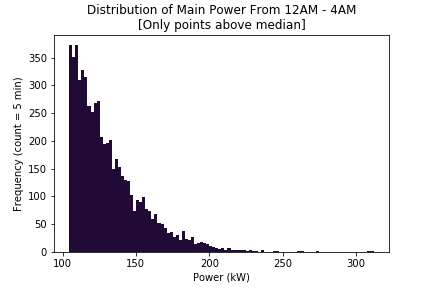
Here’s the plot of the selected data. It’s roughly a slice from the right side of the peak. This is the part of the data that I’m going to want to analyze for values that have an abnormal variation.

Unfortunately, pandas is sneaky and provides a Pandas.Series.mad() function, but it’s actually for the mean absolute deviation, not the median absolute deviation. Tomorrow I’ll see if there’s already one in existence, otherwise I’ll just make the function myself.