Day 23

The team met at the library today. I started by making a list of the items that we may want to consider working on:

• fitting a log-normal distribution to the data
• marking values past a certain percentile of that PDF
• translating data sample to match the fitted estimation
• doing something with the temperature data
• Poisson regressions
• likelihood estimation calculation, alternatively SSE

A lot of these rely on already having a fitted distribution, so that was our goal for today.

You can find the code here.

Fitting an expected distribution

At our last meeting with Viraj we discussed using a log-normal distribution as our expectation to account for the lower bound. SciPy can automatically fit() a given distribution to a dataset. At first we used the built-in scipy.stats.lognorm distribution to perform this fit, however, it was finicky to deal with and it involved extra parameters. Instead we found it easier to just take the log of our sample values and fit a scipy.stats.norm distribution to that adjusted set.

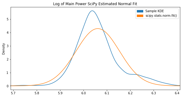
Out of the box, the fit() function didn’t achieve what we had hoped:

Apparently these parameters maximize the “likelihood estimation”, however it’s not visually close to the KDE plot.

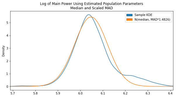
To get us closer, we scrapped the fit() approach and tried calculating our own mean and SD values by using the sample median and adjusted MAD:

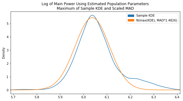
Already looking a lot better. This is pretty much where things were left off on Day 13. It’s still a bit off center though. The center we really want is essentially the peak of the KDE plot. To find this, we converted the KDE value array into a Series and found the .max(). Then based on the index of that max, we found the corresponding x value in the x-array by converting that to a Series as well. The end code is pretty ugly, but it gets the job done:

x = pd.Series(np.linspace(log_school_main.min(), log_school_main.max(), 10000))
kde = stats.gaussian_kde(log_school_main)
kde_pdf = pd.Series(kde.pdf(x))
est_mu = x[kde_pdf[kde_pdf == kde_pdf.max()].index].iloc[0]

One thing to remember is that the step count in the np.linspace() call affects the accuracy of this calculation. We tried using np.arrage() to set a fixed step size, but on larger samples it made the sample count unreasonably large causing an error at runtime.

Note: I would like to improve this implementation in the future to directly calculate the exact peak of the KDE PDF rather than an estimate. Perhaps there is some way to find the derivative of the KDE function

Now it is centered properly. It would be a better fit if there was a lower variance which could be accomlished by decreasing our scaling factor, but after tweaking the MAD scaling factor and testing various sample data sets we found the original value of 1.4826 to be the fairest overall.

Since there was some variation in the fit using this constant Frank suggested implementing some kind of dynamic scaling factor that tries to match the peak value of the KDE PDF to the estimated PDF, so that may be an area to look into.

Flagging the high points

Now that we have a expected fit density function we can calculate the value at a given percentile using scipy.stats.norm.ppf()

Then we can plug that into the scipy.stats.percentileofscore() function to get the percentile equivalent of that value from our original sample. For the Main power data during school hours, we got:

In [16]: stats.percentileofscore(log_school_main,stats.norm.ppf(0.95, est_mu, est_sd))
Out[16]: 86.532858530268697

That means that about 13.5% of the sample data is operating at power values predicted by only 5% of the expected model. That yields an 8.5% surplus of power usage in this region. Ideally there would be no difference, though I’m not yet sure what percentage difference would qualify as statistically significant. That is another area we should look into.